Tags: databricks, delta lake, big data, incremental refresh, machine learning
Incremental refresh
This paper describes what I also called temporal join in the past. Suppose you have 2 big data tables (e.g. delta tables). Because the tables are so big, they are incrementally refreshed. This means that every day we add or change only the new data and mark this with e.g. a unique timestamp. Using this timesstamp, downstream applications can pickup these changes and there is no need for an expensive full table refresh . This paper will explain how we can also use this timestamp for efficient joining.
Example data
To explain this incremental join we introduce the following example datasets:
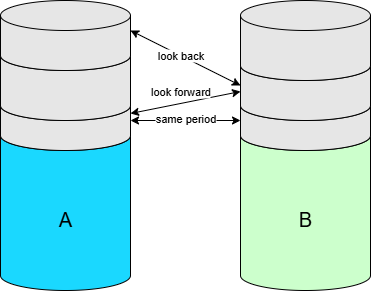
A: Bank Transactions from the financial system
B: Bank Transaction from the SEPA payment engine.
Note that both tables are huge ( like multiple terabytes) and both tables contain facts that do not change, so we only need to add new data(or facts) to A and B and we don’t need to update any historic data.
Joining incrementally refreshed tables
Suppose we want to join A with B and because both A and B are big we want to limit the scope of this join to the smallest possible dataset. The issue is however that we don’t know exactly which increment contains the matching records in B. So this is requirement 1.
Requirement 1. Join A with B where B is filtered to the smallest scope possible in order to get the best performance.
A second requirement is that we want to have a waiting mechanism for records that do not match, because the matching record in B can still arrive in the future
Requirement 2. Wait for unmatched records for a certain amount of time (called the look forward period).
However we should not wait forever, because we do not want to postpone the delivery of these unmatched records from A to the consumer
Requirement 3. If after this look foward period the match between A and B can still not be made we call this join outdated. Outdated records from A will be deliverd to the consumer. However they will not be joined with B.
The final requirement is that no matter how we process this join (e.g. per day, month or year), the outcome should always be the same, or in other words: the history of the joined data should never change. This last requirement is important when you use this data e.g. for machine learning and you don’t want to have to deal with changing data.
Requirement 4. The result of A increment join B should always stay the same, even if you reprocess this join using a larger interval ( e.g. month or year). This requirement is relevant when you reprocess the join for old data that was previously processed on a daily basis. e.g. let’s say you reprocess the year 2023 all at once. Now B contains all records of 2023. This might give a better join, but because of requirement 4 we will join as good as we did when it was daily processed. The con of this requirement is that you don’t benefit of a better match percentage when you join on a larger interval. The pro of this requirement is that your machine learning models will behave just the same because the data has not changed.
Implementation
Join scenario’s
Same period
A and B are processed in the same increment, or on the same day (assuming that an increment is a day). This is of course the happy flow and for most records this is usually the case.
A is late
A is in a newer increment than B. For example at march 6 we receive a record in A that we are expected to join with B, but the matching record in B was already present in the increment of march 2.
Look back period specifies the number of increments that we look back when trying to join A and B. (e.g. 6 days).
B is late
When we process A on march 6, B is not present yet. Only at march 10 the matching record in B is delivered.
Look forward period specifes the number of increments that we look forward when trying to match A and B. (e.g. 10 days).
Incremental join of A and B is outdated
After the lookback and lookforward we still cannot match A and B. For example: if we still did not find a match on march 16, then we send A unmatched to the output. ( because A was received on march 6 and the look forward period is 10 days).
Implementation using sql
 A left join B where
	( -- same day
		(
		  A._ProcessDate>=ProcessPeriodStart &
		  A._ProcessDate<=ProcessPeriodEnd
		) &
		( A._ProcessDate==B._ProcessDate
		)
	)
	|
	( -- A is late (for max look_back_days days) or same day
		(
		  A._ProcessDate>=ProcessPeriodStart &
		  A._ProcessDate<=ProcessPeriodEnd
		) &
		( B._ProcessDate>=date_add(A._ProcessDate, -look_back_days) &
		  B._ProcessDate<A._ProcessDate
		)
	)
	|
	( -- B is late
		(
		  B._ProcessDate>=ProcessPeriodStart &
		  B._ProcessDate<=ProcessPeriodEnd
		) &
		( A._ProcessDate>=date_add(B._ProcessDate, -look_forward_days) &
		  A._ProcessDate<B._ProcessDate
		)
	)
	|
	(  -- A is outdated ( unable to match with B).
	  A._ProcessDate>=ProcessPeriodStart-look_forward_days and
	  A._ProcessDate<=ProcessPeriodEnd-look_forward_days and
	  B._ProcessDate is null -- no match in  all period
	)
Target increment timestamp
Note that we identify each increment with a unique and sequential timestamp. When we join A with B we should define the target timestamp for the joined data.
Target timestamp for A incremental join B: Max timestamp from A and B or outdated timestamp.
Conclusion and next steps
We described a way of joining very large incrementally refreshed tables, that is focussed on performance and consistency. We moved this logic into a python function in databricks. The big advantage of this is that you remove the complexity from your code, so that you code becomes better readable. It will only contain the things that are specific for the datasets that you are joining, e.g. join condition, look back and look forward intervals and aliases for the datasets so that you will not get duplicated columns.
I am thinking about making a public library for spark to support this join type. Let me know what you think.